Lab 1 - Finite Difference

Abstract

A Python code is created to model a problem and find its solution. The finite difference method (FDM) is implemented in the code which contained methods to discretise the problem and a three point centred model is used before outlining the Neumann and Direchlet boundary conditions. Approximations were found, which were then compared to analytical solutions where the error is displayed using a log-log chart.

It is found that the centred approximation is more accurate than the backwards approximation. This confirms the theory, which states that the centred approximation should be more accurate. As the order of truncature for a centred scheme is two and for a backwards scheme its one. This will be refered to later in section 1.3.

1 Introduction

The objective is to find the approximative solution to the problem by using the Finite Difference Method (FDM) and assess its accuracy by comparing it to the analytical solution which is also calculated with Python. Therefore, the context is to verify if the approximate method is accurate enough to justify not using the analytical solution because it is calculated manually, thus taking more time.

There were three methods of identifying points used forward, backward and centred approximation. These are outlined below: An algorithm was wrote on Python using Numpy as a math function. The following steps were used to discretise the problem, the three point centred approximation was used to discretise the differential equation except the extremities. It was needed to take into account the boundary conditions in order to have a unique solution. Dirichlet is the lower boundary condition at the begining of the domain and Neumann is the upper boundary at the end of the domain.

The analytical solution was calculated to test the error in the approximate solution. The analytical solution was obtained by integrating the ODE twice and applying the boundary conditions, when the analytical solutions for the three source terms were found and inputted into the python code, they were compared to their respective approximate results. The method of comparison used was a log-log graph to represent the linear evolution of the error compared to the inverse of the grid distance.

1.1 The 1-D analysis

Figure 1: One-dimensional representation

Consider the following strong form, defined for x ∈ ]0, L[ , with L = 1:

The problem parameters K, L and qn are equal to 1. While the source term r(x) corresponds to three options:

1.2 Discretisation of the ODE

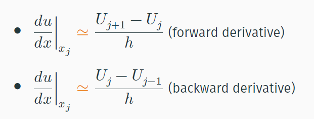
The first step of the FDM is to discretise the differential equation, a 3 point centred approximation is used. The general formula of the first derivative of a function u(x) at a general point x is:

(1)

(2)

(3)

(4)

1.3 Truncature order

In using this numerical approximation, some error must be accounted for. This is known as truncature error. Truncature error arises when certain numerical methods are used and that was the case when approximating this ODE. All error after the second order was regarded as outside of the domain of interest in this project.

(5)

(6)

The truncature error for the centered approximation is of the 2nd order.

The error was also calculated for Newmann boundary conditions in both centred and backwards boundary schemes. The order of truncature was two and one respectfully.

2 Numerical Results

Displayed below are the graphs that represent the results of the methods that were outlined in the introduction 1-D Problem section. Firstly, the approximate numerical solutions are shown for each of the three source terms, followed by the analytical algebraic solutions and finally both solutions are compared via log-log graphs.

2.1. Approximate Solutions

Below, in Figures 1, 2 and 3, the backwards and centred aproximations of the ODE 1-D problem at each of the source terms are shown. The curves were plotted for the number of points being equal to n = [10,20,40,80,160] respectively.

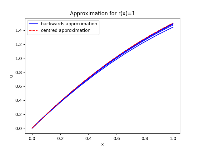
Figure 2: Approximation solution for the source term r(x) = 1

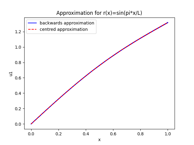
Figure 3: Approximation solution for the source term r(x)=sin(π*x/L)

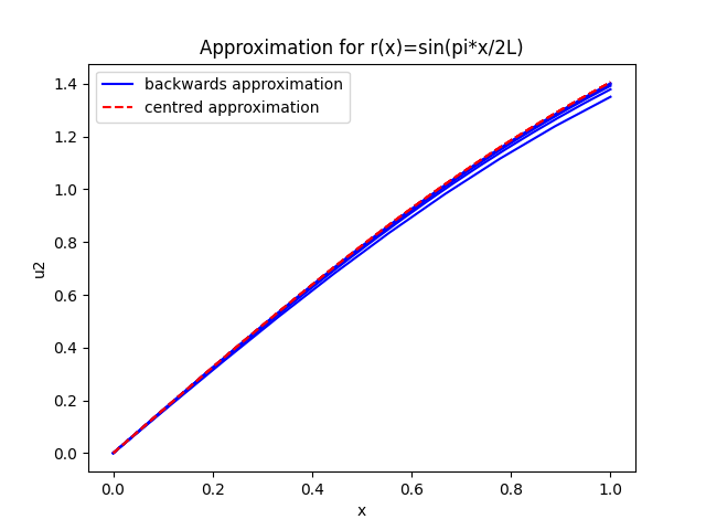
Figure 4: Approximation solution for the source term r(x)=sin(π*x/2L)

For each of the three source terms, ten curves are plotted, five being centred approximation and 5 being backwards approximation. Each of the five curves had a different number of sampling points. As mentioned above, the range was 10, 20, 40, 80, 160. It was noted that for each of the three source terms, the lowest curve was provided by the ten point sample and the gradient of the curves increased as the number of sample points increased.

2.2. Analytical Solution

The problem given is shown below:

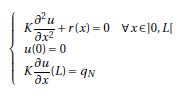
Analytical solutions for the problem were found by manually integrating the expression and subbing in each of the source terms and boundary conditions. How the solutions were obtained is showed below:

Figure 5 is the result of these solutions being solved and plotted through Python.

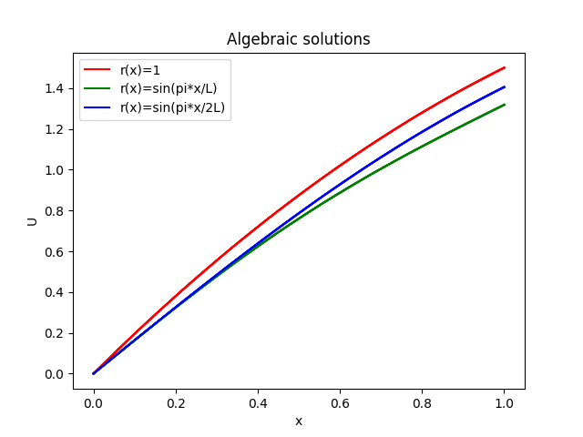
Figure 5: Algebraic solutions for the three different source terms

2.3. Error between analytical and approximation

To determine the accuracy of the approximation and to compare the backward and centered approximation, a logarithmic graph was plotted taking the absolute value of the distance between the algebric curve and the approximate curve as the ordinate and the inverse of the distance between sampling points as abscissa. The results for the three source terms are shown below.

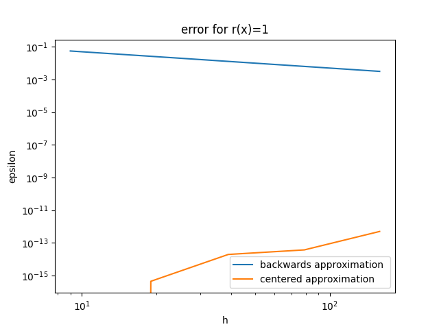
Figure 6: centred and backwards error r(x) = 1 (log-log graph)

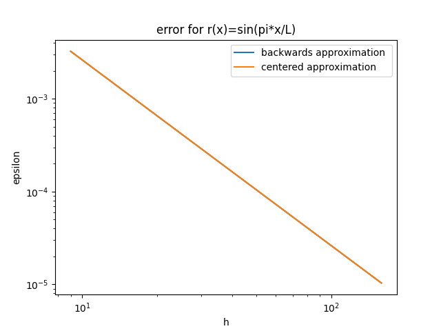
Figure 7: centred and backwards error r(x) = sin(π*x/L) (log-log graph)

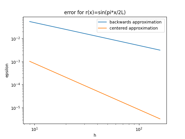
Figure 8 - centred and backwards error r(x) = sin(π*x/2L) (log-log graph)

The first source term was deemed to be the most accurate as the centred approximation was significantly lower than any other error presentented, however it also gave the most substantial difference between centred and backwards approximations.

3. Conclusions

The accuracy of the numerical methods was found to be dependant on the order of truncation of the approximation as well as the amount of points (n) chosen to be considered. For this report, a range of values of n = 10, 20, 40, 80, 160 were secected. The accuracy of the approximations increased as the value of n increased.

Source term u1, it was found that there was no difference between the centred and backwards approximations.

The truncation error theory states that the centred approximation should be more accurate than the backwards approximation because the centred approximation is second order and the backwards approximation is first order. This is confirmed in this project as for all three source terms, the centred approximantion was less than or equal to the backwards approximation.