C11BD: BIG DATA ANALYTICS 2023-2024 - INDIVIDUAL COURSEWORK 2

Introduction

The performance of a retail business is generally evaluated by analyzing their sales and profit margins over time or using predictive statistical models such as regression. This report provides an analytic insight into a retail supermarket’s current business position. Analysis has been performed in Python using potential models as time-series and linear regression. The dataset used in this analysis has several columns containing sales records for the timeframe 2014-01-03 to 2017-12-30. Based on this historical data a categorical bar graph and a continuous scatterplot has been shown during EDA along with a statistical description of the data while during forecasting sales a regression model has been employed with a time-series line plot for the predicted outcomes.

Aim and Objectives

Aim This analytic report aims to analyze the data features stored in a sales record to forecast sales for the timeframe 2017-12-31 to 2021-12-27 using linear regression and visualization of the predicted outcomes using a time-series line plot. Objectives ● To improve data quality by the removal of outliers during pre-processing of data. ● To provide the significance of a few features by means of statistical and visual interpretation. ● To forecast the sales using a linear regression model and visualize it through a time-series plot.

Research Questions

Research Question 1: Detect the outliers in data to improve its quality. Research Question 2: Provide feature significance by statistical description and plotting of a categorical bar graph and a continuous scatterplot. Research Question 3: Forecast sales for the supermarket during the timeframe of 2017-12-31 to 2021-12-27 using linear regression. Visualize the predicted outcomes using a time-series line plot to show whether the predicted sales are increasing or decreasing.

Background

Mathematical and statistical models often turn out to be potential tools for analyzing market positions of a retail business. Linear regression is a statistical model that is usually used in case of continuous data and sales prediction. The forecasting of sales indicates the future market position of a company by means of business growth. Business growth of a company depends on operational sustainability which on the other hand relies on market demand (Ma and Fildes, 2021). For manufacturing businesses, when the rate of production is more than the rate of consumption of a product of high demand, it is said that sustainability is maintained. According to Teoh and Rong, 2022, on the other hand, for a retail business such as supermarkets, sustainability is maintained only if the business manages to balance the “economic”, “environmental”, and “social concerns” without disrupting the chain of market demand and selling of products. The conservation of this sustainability needs thorough knowledge of the current market state. In order to introduce stability in business operations, retail businesses often employ data analysts to provide valuable information of the current situation and expected growth or contraction in businesses. Analysts use business records of their employers to describe current business state and based on which they show whether a business is likely to grow or otherwise (Bauer et al., 2022). Based on such analyses, business strategists plan future aspects to improve the current situation.

Methods

This research is directed to provide the same for the organization which has generated this “Superstore.csv” record on their sales performance. The methodical approach begins with the pre-processing of the data to remove the outliers from the dataset. The analysis proceeds to portray a statistical description of data to show the measures of central tendencies of each variable involved. It further produces a pair of graphs - a categorical bar plot showing the data distribution of a categorical column present in the dataset and a continuous scatterplot showing any dependencies between two indicators of current market status of an organization. Forecasting of sales records has involved the application of a linear regression model while the observation of the predicted sales incorporates a time-series analysis using a line plot. The entire analysis has been performed in Python using a few of its pre-defined functions. Python provides a diverse functionality for prediction models that can be acquired from the “scikit-learn” library. “Pandas”, on the other hand, is a library that makes data handling more flexible and structured with the dataframe-like tabular structure of data and many functions for data type conversion, and operations like merging and joining (Fan et al., 2020). The library “scikit-learn” allows access to regression models that are pre-defined in the “sklearn.linear_models” modules (Prell et al., 2020). The performance metrics for regression models incorporate the measuring of “mean absolute error”, “mean square error”, and “root mean square error” that define the error margin of a regression model (Smiti, 2020). Low error margin indicates greater model accuracies. The linear regression model applied to forecast the sales for the period 2017-12-31 to 2021-12-27, has a general form as follows. y = mx + c Here, “y” is the predicted sales and the response variable that depends on the “x” which is the predictor variable while “c” is the constant term. For a known set of values of x and y, “m” and “c” are calculated first, then for each known value of the predictor, m and c, the values of “y” are produced as predicted outcomes of sales.

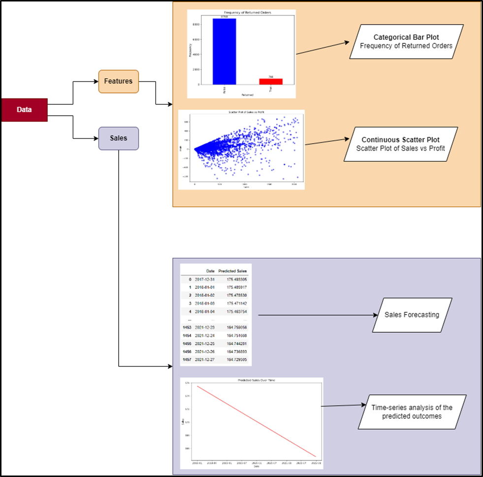
Methodical implementation plan (Source: Designed in draw.io) The implementation plan thus includes the removal of the outliers, feature analysis and forecasting using a linear regression model with an aim to predict the future market position of the company.

Implementation, Results and Discussion

The dataset for analysis has been loaded into the programming environment with the use of the “read_csv()” function. The function takes the name of the dataset along with its file extension as a positional argument along with other parameters specifying the file encoding, data separator, presence of headers, and so on. The loaded data has a dataframe structure supported by the “Pandas” library.

The dataframe is appeared to have 9994 rows, 29 columns and 289797 observations with no null values. There are four types of data present in the dataset are “bool”, “float64”, “int64”, and “object” associated to 1, 3, 10, and 15 columns. Among the columns “Order Date”, “Customer Name”, “Postal Code”, and so on, the column “Sales” is the target column.

Followed by the loading and description of the dataframe, pre-processing has been performed during which the outliers from the dataset have been detected first as the adjacent figure illustrates. The computation of z-score has helped to identify the outliers - those data points that are scattered at a great distance from the overall mean position of the data points (Alghushairy et al., 2020). The statistical tool, namely “standard deviation”, has been employed during the evaluation of z-scores to measure the distances between each data point from the aforementioned mean position. The data points situated at a greater distance from the mean position, i.e. those having greater “standard deviation” are considered to be outliers. The user-function used in this case calculates the z-scores for all data points and returns the location or indices of those data that have greater SD. The result of the adjacent block of code shows there are a total of 460 outliers present in the dataset along with their indices. Using Python’s pre-defined “drop()” function these outliers are removed from the dataframe to reduce data noise and improve data quality.

The statistical description of the dataframe uses only numeric and date-time columns to calculate the measures of central tendencies of each data point. The mean sales, quantity of goods sold, and profit of the company have appeared to be $180.53, 3.7, and $23.56 respectively. This indicates, by selling an average of 3.7 products, the supermarket makes a sale of $180.53 while manages to gain $23.56. On the other hand, as the average order and shipping date are “2016-04-30 17:09:28.659534336” and “2016-05-04 16:02:34.059156736”, the supermarket delivers goods to their customers on an average delay of 3 days approximately.

The “Returned” column stores binary data - “True” and “False” - indicating whether a certain product is returned by a customer or not. While “False” indicates “no order is returned”, “True” refers to the returned orders. Thus a distributed count of the occurrences of these values indicates total orders returned and not returned. As bar plot illustrates, on selling 9534 products, 766 of them are returned by the customers.

The relational dependency of sales on profit has been described on the adjacent figure. By plotting the sales on x-axis and profit on y-axis the data points have formed a clustering that appears to be diverging from the coordinate (0,0). The cluster is denser at the origin indicating the difference between the profit and sales are very low. The dense cluster has spread more on the positive quadrant while a minimal portion is on the negative quadrant. This implies besides making low profits, the organization also faces losses. Those data points that are situated far from this cluster are the residues of outliers still present in the data. A trace of a linear dependency is found for these two variables within the range [0, 600) though the line has seem to lose its consistency at the coordinate of (1500, 300).

Linear regression fits a straight line to training data, modeling the relationship between independent variables (features) and a dependent variable (target). It recognizes the straight relationship by minimizing the distinction between anticipated and genuine values. The code likely utilizes X_train as highlight inputs and y_train as target values. Once trained, the model predicts target variables for new data points. This method is fundamental for understanding and predicting relationships between variables in various fields, from economics to machine learning.

The above implementation has utilized Python libraries like NumPy and Pandas to foresee future deals (sales_predicted) based on historical data (df_filtered). It forecasts sales for the next 1459 days (days_next). Referring to a "thermometer" allegorically, it can signify a factual show for deals forecast, serving as a gauge to measure deal patterns. This strategy helps in expecting future sales patterns and making informed decisions in business planning and strategy.

The Python code produces a Pandas DataFrame with the title predicted_df. It contains two columns: 'Date' which ranges from December 31, 2017, to December 27, 2021, and 'Predicted Sales' which shows deals insights that connect to the dates. There are 1458 rows of data contained inside the DataFrame.

Based on the above results the mean absolute error has been shown as 169.05 and on the other hand the root mean error is defined as 235.34. The code assesses the execution of the model by comparing predicted values with real values. The resulting metrics are shown in the code, providing bits of knowledge about the accuracy and performance of the model.

A line graph is used to illustrate "Predicted Sales Over Time" from January 2018 to July 2022. There is a small rising trend in the sales data along the y-axis, however there is some variability.

Conclusion

The analytic report has confirmed that the company running the supermarket is likely to face a loss during the forthcoming period of 2017-12-31 to 2021-12-27. The company has gained minimum profits during the period 2014-01-03 - 2017-12-30 with decreasing trend of sales. It purchases products from third parties and sells them at an average profit of $23.56. It also has made a loss of $653.28 during the timeframe under observation. With an average delay in delivery of 3 days, the company receives 799 returned orders while selling a total of 9,534 products. The loss for the company during the upcoming time has been predicted to fall below $166 at the end of 2022 starting from $176 at the beginning of 2018.

References

Alghushairy, O., Alsini, R., Soule, T. and Ma, X., 2020. A review of local outlier factor algorithms for outlier detection in big data streams. Big Data and Cognitive Computing, 5(1), p.1. Smiti, A., 2020. A critical overview of outlier detection methods. Computer Science Review, 38, p.100306. Ma, S. and Fildes, R., 2021. Retail sales forecasting with meta-learning. European Journal of Operational Research, 288(1), pp.111-128. Teoh, T.T. and Rong, Z., 2022. Python for Data Analysis. In Artificial Intelligence with Python (pp. 107-122). Singapore: Springer Singapore. Bauer, J.M., Aarestrup, S.C., Hansen, P.G. and Reisch, L.A., 2022. Nudging more sustainable grocery purchases: behavioural innovations in a supermarket setting. Technological Forecasting and Social Change, 179, p.121605. Prell, M., Zanini, M.T., Caldieraro, F. and Migueles, C., 2020. Sustainability certifications and product preference. Marketing Intelligence & Planning, 38(7), pp.893-906. Fan, Y., Kou, J. and Liu, J., 2020, January. Research on the influencing factors of customer loyalty in offline supermarket under new retail model. In Proceedings of the 2020 4th International Conference on Management Engineering, Software Engineering and Service Sciences (pp. 216-220).