trabajo realizado en el ciclo 2023-II. Profesor: Jeronimo Garcia
import pandas as pd
import numpy as np
from numpy import pi, cos, sin, tan
import pandas as pd
df=pd.read_csv("/work/data_temp_rad.csv")
df
# Convertir la columna 'Fecha_Hora' a objetos datetime
df['TIMESTAMP'] = pd.to_datetime(df['TIMESTAMP'], format="%m/%d/%Y %H:%M")
# Crear nuevas columnas 'Fecha' y 'Hora'
df['Fecha'] = df['TIMESTAMP'].dt.date
df['Hora'] = df['TIMESTAMP'].dt.time
# Mostrar el DataFrame resultante
df
df.dtypes
temperatura_maxima_por_dia=df.groupby(df['TIMESTAMP'].dt.date)['T_Avg'].max()
temperatura_min_por_dia=df.groupby(df['TIMESTAMP'].dt.date)['T_Avg'].min()
# temperatura_mean_por_dia=df.groupby(df['TIMESTAMP'].dt.date)['T_Avg'].mean()
Slr_wm=df.groupby(df['TIMESTAMP'].dt.date)['SlrRad_Wm2_Avg'].sum()
df['T_Avg'] = pd.to_numeric(df['T_Avg'], errors='coerce')
temperatura_mean_por_dia=df.groupby(df['TIMESTAMP'].dt.date)['T_Avg'].mean()
temperatura_mean_por_dia
temperatura_min_por_dia
Slr_wm
df_2=pd.DataFrame({'Fecha': temperatura_maxima_por_dia.index, 'TMax': temperatura_maxima_por_dia.values,
"Tmin":temperatura_min_por_dia,"Tmedia":temperatura_mean_por_dia,"Rad_inc_acc_w_m2":Slr_wm})
df_2
# Crea un rango de fechas
fecha_inicio = "2023-09-21"
fecha_fin = "2023-12-22"
# Convierte las columnas de fechas a tipo datetime si no lo están
df_2['Fecha'] = pd.to_datetime(df_2['Fecha'])
# Realiza el subconjunto de las fechas en el rango especificado
df_3 = df_2.loc[(df_2['Fecha'] >= fecha_inicio) & (df_2['Fecha'] <= fecha_fin)]
df_3
# Convierte la columna 'TMax' a tipo numérico
df_3['TMax'] = pd.to_numeric(df_3['TMax'], errors='coerce')
df_3['Tmin'] = pd.to_numeric(df_3['Tmin'], errors='coerce')
# df_3['Rad_inc_mean'] = pd.to_numeric(df_3['Rad_inc_mean'], errors='coerce')
df_3["tmean"]=(df_3["TMax"]+df_3["Tmin"])/2
df_3
Calculo de la qi (segun Formula Garcia)
#Hallando Theta
Na = df_3['Fecha'].dt.strftime('%j').astype(float)
theta = Na*2*np.pi/365
#Hallando angulo de declinacion solar
decl = (0.00692-3999.12*np.cos(theta)+702.57*np.sin(theta)-67.58*np.cos(2*theta)+9.08*np.sin(2*theta))*10**-4
#Hallando la relación de distancia media (dm) e instantanea (d) entre el Sol y la Tierra
dist = 1.00011+0.033523*np.cos(theta)+0.00128*np.sin(theta)+0.000739*np.cos(2*theta)+0.000099*np.sin(2*theta)
#Hallando angulo horario a la salida del sol
#La latitud del OVH se encuentra en el sur, por ello negativo
L= -12.01
H = np.arccos(-np.tan(L*np.pi/180)*np.tan(decl*np.pi/180))
H = H*180/(np.pi)
#calculando fotoperiodo del sol
N = (2*H)/15
#Calculando ángulo zenital
Z = np.arccos(sin(L*pi/180)*sin(decl)+cos(L*pi/180)*cos(decl)*cos(H*pi/180))
Z = Z*180/pi
#dQs
S = 1395
dQs = S*(dist)*cos(Z*pi/180)
###Temperaturas###
#TEMPERATURA MINIMA
Tmin=df_3['Tmin']
#TEMPERATURA MAXIMA
Tmax=df_3['TMax']
# Rango térmico (°C)
dT=Tmax-Tmin
### Radiación incidente ###
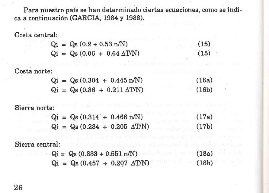
Qi = dQs*(0.06 + 0.64*dT/N) # En mm/día
df_3["Qi_garcia"]=Qi
Sv=0.858
Qsv=458.37*Sv*dist*(((H*np.pi/180)*np.sin(L*(np.pi)/180)*np.sin(decl)) + (np.cos(L*(np.pi)/180)*np.cos(decl)*np.sin(H*np.pi/180)))
df_3['Qsv'] = Qsv
df_3
df_3['qi_ly_day'] = df_3["Rad_inc_acc_w_m2"]*0.484583/24
df_3
#UTILIZANDO TEMPERATURAS PARA TEMPERATURA PROMEDIO EN EL DIA
Tavg = df_3['Tmedia']
#hallando to
to = 12 - 0.5*N
to
#TEMPERATURA PROMEDIO DIURNO
Tmd = Tavg + ((((Tmax-Tmin)*(11+to))/(12.56*(12-to)))*np.sin((np.pi/180)*((11-to)/(11+to))))
df_3 = df_3.assign(Tmd = Tmd)
#Parametro que indica el grado de cobertura nubosa del cielo
F= (df_3["Qsv"] - 0.5*df_3["Qi_garcia"])/(0.8*df_3["Qsv"])
df_3["F"]=F
df_3
df_3["n_dias"]=[*range(1,len(df_3.Fecha)+1)]
interpolación de PM
bo=[]
bc=[]
#Para el bo y bc según la tabla
for i in np.arange(0,len(df_3.Fecha),1):
if df_3.Fecha.dt.month.iloc[i] ==9:
bc_m = 418
bo_m = 223
bo.append(bo_m)
bc.append(bc_m)
elif df_3.Fecha.dt.month.iloc[i] ==10:
bc_m = 437
bo_m = 234
bo.append(bo_m)
bc.append(bc_m)
elif df_3.Fecha.dt.month.iloc[i] ==11:
bc_m = 440
bo_m = 238
bo.append(bo_m)
bc.append(bc_m)
elif df_3.Fecha.dt.month.iloc[i] ==12:
bc_m = 446
bo_m = 238
bo.append(bo_m)
bc.append(bc_m)
df_3["bo"]=bo
df_3["bc"]=bc
import numpy as np
import matplotlib.pyplot as plt
# Tus listas de datos
tmd_x_datos = [4,5, 7.5, 10, 15, 15.5,16,20,22.5,25,27.5,30,35]
pm_datos = [4,5, 10, 15, 20, 20.5,21,20,19,18,15,10,5]
# Crear la función de interpolación polinómica
polinomio_interpolacion = np.polyfit(tmd_x_datos, pm_datos, deg=3)
p = np.poly1d(polinomio_interpolacion)
# Generar nuevos datos para la curva interpolada
x_interpolacion = np.linspace(min(tmd_x_datos), max(tmd_x_datos), 1000)
y_interpolacion = p(x_interpolacion)
# Graficar los datos originales y la curva interpolada
plt.scatter(tmd_x_datos, pm_datos, label='Datos originales')
plt.plot(x_interpolacion, y_interpolacion, label='Curva interpolada', color='red')
plt.legend()
plt.xlabel('Temperatura media (Tmd)')
plt.ylabel('velocidad fotosintetica (pm)')
plt.title('Curva de Interpolación')
plt.grid()
plt.show()
# Grado del polinomio de interpolación
grado_polinomio = 3
# Crear la función polinómica a partir de los coeficientes
polinomio_funcion = np.poly1d(polinomio_interpolacion)
# Imprimir la ecuación del polinomio
print(f'Ecuación del polinomio de interpolación (grado {grado_polinomio}):')
print("y= ",polinomio_funcion)
#Para el Pm: Pm = a(Tmd**2) +b*Tmd + c
Ec=polinomio_funcion
#Funcion parabolica de Pm
Pm=Ec[3]*df_3['Tmd']**3++Ec[2]*(df_3['Tmd']**2) + Ec[1]*df_3['Tmd'] + Ec[0]
df_3['Pm']=Pm
df_3
#Hallando la velocidad máxima de producción de biomasa bruta (bmg)
#Se utiliza IAF = 5
for i in np.arange(0,len(df_3.Pm),1):
if df_3.Pm.iloc[i] <20:
bmg = (df_3.F*df_3.bo*(1-0.025*(20-df_3.Pm))+df_3.bc*((1-df_3.F)*(1-0.005*(20-df_3.Pm))))
elif df_3.Pm.iloc[i] >20:
bmg = (df_3.F*df_3.bo*(1+0.025*(df_3.Pm-20))+df_3.bc*((1-df_3.F)*(1-0.001*(df_3.Pm-20))))
df_3['bmg'] = bmg
df_3.Pm
df_3
Run the app to see this chart
Press the run button in the top right corner
import seaborn as sns
import matplotlib.pyplot as plt
sns.set_style("darkgrid")
f, ax = plt.subplots(figsize=(7, 5))
sns.lineplot(x=df_3.index,y="bmg",data=df_3,marker="o", label="bmg")
ax.set_title("Variacion temporal del bgm")
ax.set_ylabel("produción de biomasa bgm")
ax.set_xlabel("Fechas")
ax.legend()
# Rota las etiquetas del eje x 90 grados hacia arriba
#ha= center, para que se alinien hacia el centro
plt.xticks(rotation=90, ha='center')
# # Agrega los valores de cada dato
# for index, value in enumerate(iaf["IAF"]):
# plt.text(index, value, str(value), ha='center', va='bottom')
# # plt.text()
plt.tight_layout()
plt.savefig("iaf.png")
Ct=0.0108*(0.044+0.0019*df_3["Tmedia"]+0.001*(df_3["Tmedia"]**2))
#CALCULANDO LA BIOMASA NETA (Bn)
Bn = (0.36*bmg*df_3["n_dias"])/(1+0.25*Ct*df_3["n_dias"])
df_3['Bn']= Bn
df_3["Ct"]= Ct
df_3
Run the app to see this chart
Press the run button in the top right corner
df_3
Run the app to see this chart
Press the run button in the top right corner
Run the app to see this chart
Press the run button in the top right corner
Run the app to see this chart
Press the run button in the top right corner
Run the app to see this chart
Press the run button in the top right corner
se puede mejorar la Tmedia del aire
bn_exp=pd.read_csv("/work/bn_experimental1.csv")
import pandas as pd
# Tus nuevos datos
data = {
'fecha': ['13/10/2023', '17/10/2023', '23/10/2023', '28/10/2023', '29/10/2023', '3/11/2023', '7/11/2023', '20/11/2023', '12/12/2023'],
'dias': [22, 26, 32, 38, 39, 43, 47, 60, 82],
'Masa seca': [0.0425, 0.045, 0.101287554, 0.4, 0.41, 0.645, 0.56, 0.759, 0.69689505],
'bn': [283.3333333, 300, 675.2503573, 2666.666667, 2733.333333, 4300, 3733.333333, 5060, 4645.966997]
}
# Crear un DataFrame
df = pd.DataFrame(data)
# Mostrar el DataFrame
df
df["fecha"]=pd.to_datetime(df["fecha"],format="%d/%m/%Y")
df["bn"]=df["bn"]/2 #para pasar a 30 cm2 como area por planta
import matplotlib.pyplot as plt
fig,ax=plt.subplots(1,1,figsize=(10,6))
ax.set_ylabel("Produción de biomasa bgm $kg/ha.día")
ax.set_xlabel("Fechas")
ax.plot(df_3["Fecha"],df_3["Bn"],label="Biomasa neta (Bn) modelo")
ax.plot(df["fecha"],df["bn"],marker="o",label="Biomasa neta (Bn) muestreo \n semanal")
ax.legend()
# Ajustar el formato de las fechas en el eje x
plt.xticks(df_3['Fecha'][::7], rotation=90, ha='right') # Muestra una fecha cada 7 días
# plt.xticks(df['fecha'][::7], rotation=90, ha='right')
plt.suptitle("Variacion temporal del productividad neta acumulada",weight="bold")
plt.savefig("bn_exp.png")