DS510 - Final Project

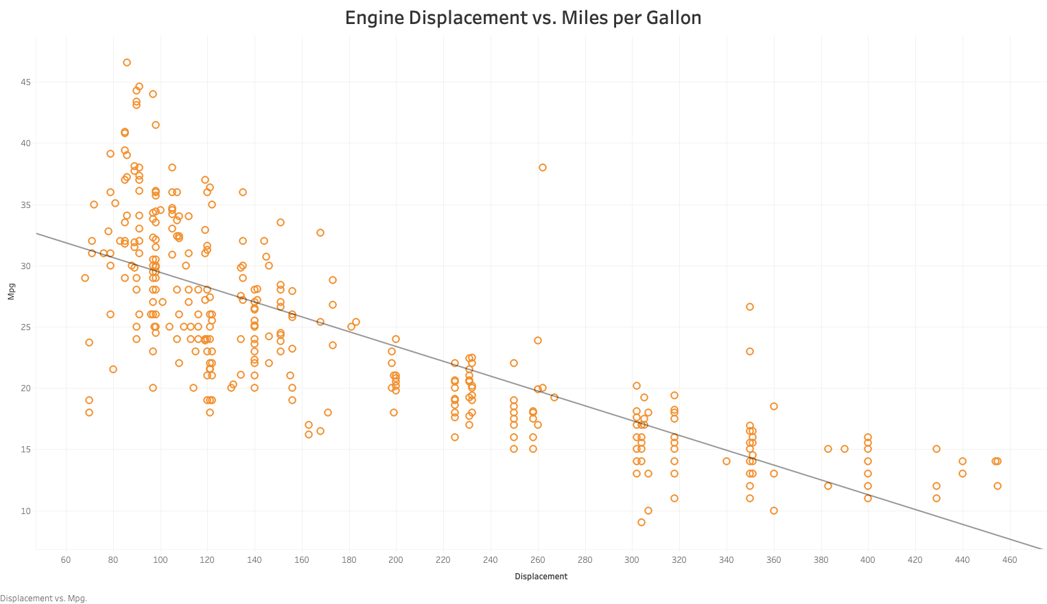
The chart above showcases the relationship between engine displacement and the miles-per-gallon autonomy of a car. As we can see from this chart, vehicle efficiency tends to be inversely correlated with engine size (displacement).

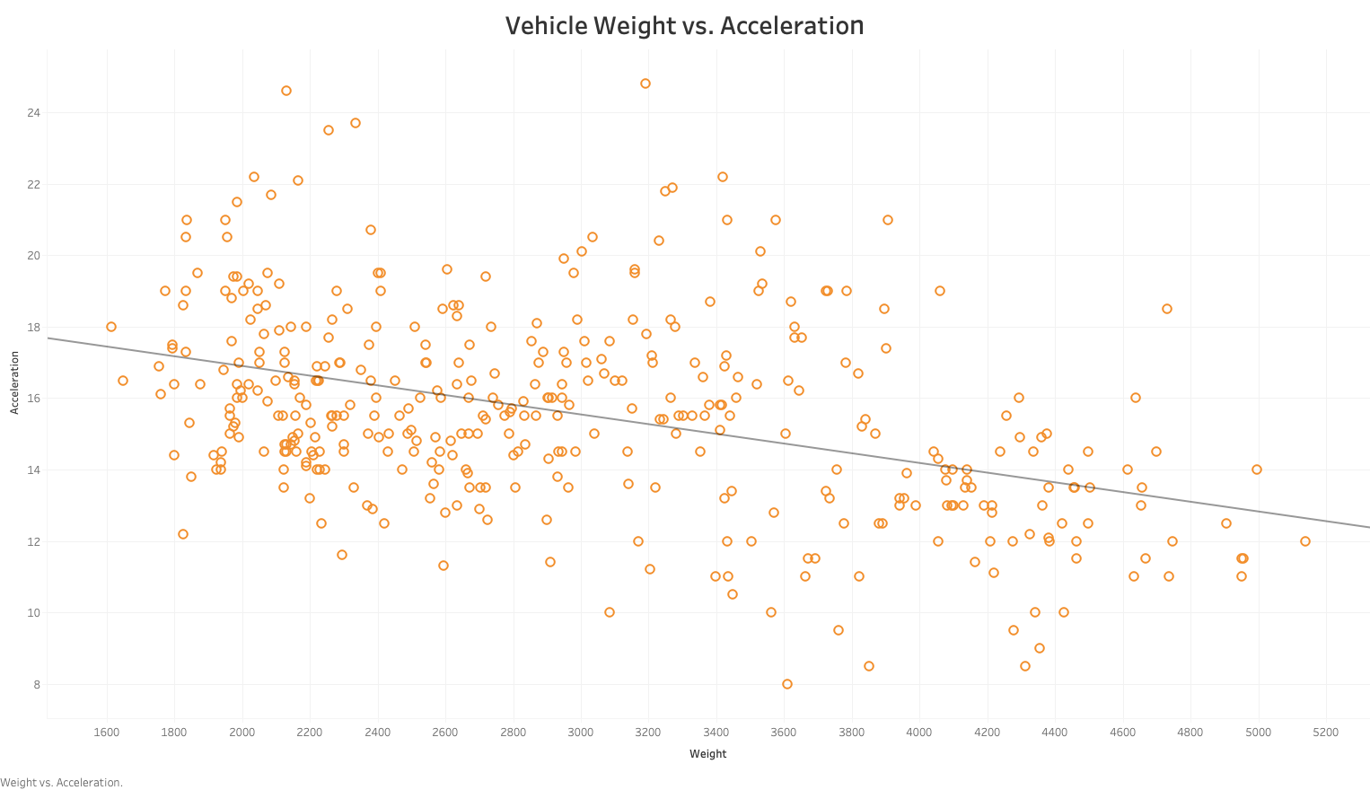
The chart above describes the relationship between vehicle weight and acceleration. As expected, we can see that a vehicle's acceleration is inversely correlated to the weight of the vehicle.
Dataset
# Read CSV file into a data frame
data <- read.csv("ds510_mpg.csv", header = TRUE, col.names = c("mpg", "cylinder", "displacement", "horsepower", "weight", "acceleration", "model_year", "origin", "car_name"))
data
Multiple Linear Regression Analysis
# Read CSV file into a data frame
data <- read.csv("ds510_mpg.csv", header = TRUE, col.names = c("mpg", "cylinder", "displacement", "horsepower", "weight", "acceleration", "model_year", "origin", "car_name"))
# Create a subset of the data frame of only the first 300 records
data <- data[1:300, ]
# Drop specified columns given categorical nature
columns_to_drop <- c("origin", "car_name")
data <- data[, !(names(data) %in% columns_to_drop)]
# Change model_year format from YY to YYYY
data$model_year <- as.numeric(paste0("19", data$model_year))
# Change the data type of the "horsepower" column to integer
data$horsepower <- as.integer(data$horsepower)
# Display the first few rows of the data
#head(data)
#Simple Linear Regression Analysis
m_cylinder <- lm(mpg ~ cylinder, data = data)
m_dis <- lm(mpg ~ displacement, data = data)
m_hp <- lm(mpg ~ horsepower, data = data)
m_weight <- lm(mpg ~ weight, data = data)
m_accel <- lm(mpg ~ acceleration, data = data)
m_year <- lm(mpg ~ model_year, data = data)
summary(m_cylinder)
summary(m_dis)
summary(m_hp)
summary(m_weight)
summary(m_accel)
summary(m_year)
# Multiple Linear Regression Analysis based on coefficients which had the strongest correlations in prior analysis
model <- lm(mpg ~ cylinder + displacement + horsepower + weight + acceleration , data = data)
# Display summary of the regression model
summary(model)
# Display Multiple Linear Regression Equation
cat("Linear Regression Equation:\n")
cat(paste("mpg =", round(coefficients(model)[1], 4)))
for (i in 2:length(coefficients(model))) {
cat(paste("+ (", round(coefficients(model)[i], 4), "*", names(coefficients(model)[i]),")"))
}
cat("\n")
# Read CSV file into a data frame
data_test <- read.csv("ds510_mpg.csv", header = TRUE, col.names = c("mpg", "cylinder", "displacement", "horsepower", "weight", "acceleration", "model_year", "origin", "car_name"))
# Use the model to predict mpg for the remaining 98 samples
data_test <- data_test[301:398,]
columns_to_drop <- c("origin", "car_name","model_year")
data_test <- data_test[, !(names(data_test) %in% columns_to_drop)]
data_test$horsepower <- as.integer(data_test$horsepower)
# Predict mpg using the trained model
predicted_mpg <- predict(model, newdata = data_test)
#create data frame of actual and predicted values
values <- data.frame(actual=data_test$mpg, predicted= predicted_mpg)
#plot predicted vs. actual values
plot(x=values$predicted, y=values$actual,
xlab='Predicted Values',
ylab='Actual Values',
main='Predicted vs. Actual Values - Test Sample')
#add diagonal line for estimated regression line
abline(a=0, b=1)
# Calculate residuals
residuals <- data_test$mpg - predicted_mpg
#Residual Plot
par(mfrow = c(1, 2)) # Set up a 1x2 plotting grid
plot(predicted_mpg, residuals, main = "Residual Plot", xlab = "Predicted MPG", ylab = "Residuals", pch = 16, col = "blue")
abline(h = 0, col = "red", lty = 2) # Add a reference line
#Histogram of Residuals
hist(residuals, main = "Histogram of Residuals", xlab = "Residuals", col = "lightblue", border = "black")
Model Results:
Multiple Linear Regression Equation:
mpg = 41.0054+ ( -0.248 * cylinder )+ ( -0.0029 * displacement )+ ( -0.026 * horsepower )+ ( -0.0046 * weight )+ ( -0.0615 * acceleration )
Multiple R-squared: 0.7836
Adjusted R-squared: 0.7799 --> The explanatory variables explain > 78% of the response variable's behavior (mpg)
F-statistic: 211.5 on 5 and 292 DF
p-value: < 2.2e-16 --> Highly significant, at least, one of the predictor variables is significantly related to the outcome variable (mpg)
Conclusions:
Since the model was trained on the first 300 records of the dataset, it was able to obtain a very high r-squared metric, indicating it was able to predict the miles per gallon of the vehicle with pretty good accuracy. Unfortunately, as showcased by the residual plots, the model lacks accuracy when tested on the last 98 records of the dataset. The reason for this being is that the model year of vehicles increased throughout the dataset, hence reflecting the technological advances in the automotive industry during this period. Therefore, the data that our model was trained on, doesn't account for the efficiency gains vehicles obtained as the years passed.