Neurons, Pixels, and Decisions: The Art of Neural Networks

Chapter 1. Neurons 101: From Decisions to Outputs

Imagine you're Sampy... you've got hundreds of students, everyone turning in assignments at different times, contributing to class and different ways, all while trying to run your beloved theatre class. Now, of course, to track each student's progress, you've got you're trusty rubric--a system to make decisions objectively. But, what if, instead of grading your students manually, you designed a "neural instructor" to help decide who passes and who doesn’t?

The Input

Let's say that to pass STEM and the Stage, we want to analyze three parts of a student's performance:

1. Class Participation: A score that reflects how often a student raises their hand or adds value to class discussions.

2. Assignments: The backbone of the class. Students' ability to demonstrate their understanding through projects and homework.

3. Projects: How students apply their knowledge creatively and practically, showcasing deeper understanding.

ENGAGEMENT: To test how well Han is doing in his class, use the sliders below!

But you know, not all categories are created equal. Assignments weigh the most heavily because they prove hard work and comprehension. Participation matters too, but not as much. And projects, while still important, are more about application and creativity.

So... how do we do this?

Well, out of 10, let's weigh the importance of each category accordingly!

The Bias

But wait... what's a "bias slider?" Well, that kind of depends on how Sampy is feeling today. Is he feeling a bit more lenient today? For us students, that's great! Has he been having a bad day today? Uh-oh? Being cooked isn't ideal, is it?

Remember, the more positive bias you give, the better the curve in the class. The more negative bias you give, the worse the curve. I certainly hope there won't be a negative bias, but I guess if a teacher theoretically thought all the grades in her class were too high, they could "push them back down," right?

Play with this yourself. If Sampy just had a great sandwich, there might be a positive bias. Suppose, Han's total score from class participation, turning in assignments, and

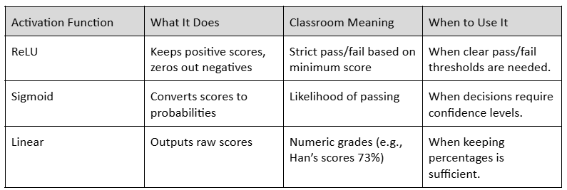
The Activation Functions

What are activation functions? In simple, they determine how the final weighted sum (percentage score) is interpreted into a decision (pass or fail).

There are 3 types:

1. ReLU:

If the score is above 0%, it stays as is. If the score is below 0%, it becomes 0, which effectively means the student fails. If the final score is 73%, ReLU outputs 73% (Han passes). If the final score is 50%, ReLU outputs 0% (Han fails outright).

Why Use It: It’s simple and mirrors hard thresholds often used in grading systems.

2. Sigmoid:

A final score of 85% might map to 97%, meaning Han has a 97% confidence of passing. A final score of 69% might map to 75%, meaning Han is borderline.

Why Use It: Sigmoid introduces nuance, useful for decisions requiring probabilities instead of absolutes. It’s like saying, "Alex has a high chance of passing but isn’t guaranteed."

3. Linear Activation:

If Alex scores 73%, Linear outputs 73%. If Alex scores 50%, Linear outputs 50%.

Why Use It: It’s straightforward and keeps the score in a format you can compare directly against the passing threshold.

Choosing the Right Activation

Each activation function serves a different purpose, depending on how you want to interpret the scores:

Check out this cell below!

How do you think Sampy will decide if Han passes the class if he gets a different weighted sum (grade) in the class? Play around below!

Calculations:

Will Han pass this class?

Chapter 2. Neural Networks: Connecting the Dots

Once again, let's imagine you're Sampy, grading a student on their performance in three categories: class participation, assignments, and projects. You might weigh each category differently—maybe participation is less important, while assignments and projects carry more weight. Then you add a bit of leniency (a bias) based on how generous you’re feeling today, and finally, you decide whether the student passes or fails. This is what we've discussed in chapter 1. But more importantly, this is, at its heart, what a neuron in a neural network does: it combines inputs (scores) with weights (importance), adjusts the result with a bias, and produces an output.

But what if you’re grading not just one student but a whole class? What if each student has scores in multiple subjects, and you want to make connections between their performances in these subjects? That’s where neural networks come in—they’re layers of interconnected neurons working together to process information.

Section 1. The Neuron as a Building Block

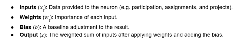
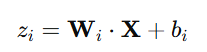
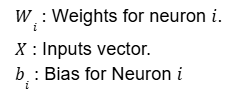
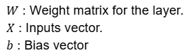
A neuron in a neural network is a mathematical function that combines inputs (𝑥) with weights (𝑤) and biases (𝑏), applies an activation function, and produces an output (𝑧).

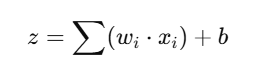
For example:

Inputs: Class Participation = 90, Assignments = 85, Projects = 80. Weights: Importance of Participation = 0.4, Assignments = 0.3, Projects = 0.3. Bias: +5 (leniency).

The neuron thus calculates:

Assuming the ReLU activation function (see ch. 1), the final output is (0,𝑧), so this student would score 90.5 (thanks to that 5 extra leniency points!)

Section 2. Connecting Neurons to Build a Network

How do neurons work together?

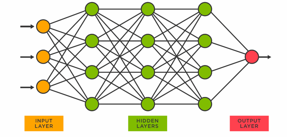
In a neural network, a single neuron is powerful but limited—it processes one set of inputs and produces one output. To solve more complex problems, we connect multiple neurons into layers to build a network. These layers are the backbone of neural networks, allowing them to learn patterns and relationships in the data.

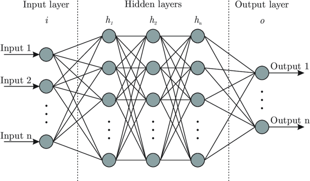
Note - Each dot in the diagram is a neuron, the mathematical function which, in our example from chapter 1, calculated the final grade of one student.

What Are Layers in a Neural Network?

A layer is a group of neurons that work together to process inputs and produce outputs:

1. Input Layer: This is the starting point, where raw data (like test scores or pixel intensities from an image) enters the network. Each input corresponds to one "node" in the input layer.

2. Hidden Layers: These layers sit between the input and output layers. Each hidden layer transforms the data further, enabling the network to detect patterns or features in the inputs. For example:

3. Output Layer: This layer produces the final result of the network's computations, such as:

Each layer takes the output of the previous layer as its input, processes it using its neurons, and passes the result to the next layer.

How Layers Interact: A Simple Example

Let’s extend our “grading a class” example:

Inputs: A student has scores for participation, assignments, and projects. Class Participation = 90 Assignments = 85 Projects = 80

Hidden Layer: Imagine we have three neurons in this layer, each evaluating a different aspect of the student's performance:

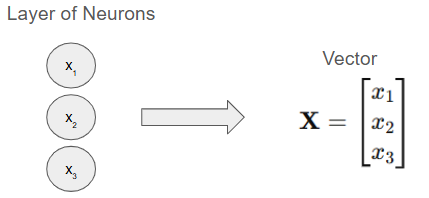
For a single layer, the output of each neuron is:

For multiple neurons, the outputs form a vector:

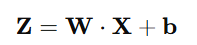
Now imagine multiple layers! What you see above is a single layer, but the next layer would be the same, except, its input is the output, Z, of the previous layer!

Real-World Application: Grading All Students

Going back to our example, imagine you're grading an entire class, not just one student. Each student's scores are inputs to the network. Here's how a neural network would process this data:

1. Input Layer: Each student's scores are represented as a vector, e.g., [90,85,80].

2. Hidden Layer: Each neuron in the hidden layer focuses on detecting patterns or features in the students' scores.

3. Output Layer: Produces a final score or decision (e.g., pass/fail) for each student.

So what's the point?

With a neural network, essentially a combination of layers, the scores of many students can be evaluated simultaneously, finding complex relationships between their performance in different categories. The neural network essentially creates a set of mathematical patterns that help us determine the combination of weights that will produce a certain output.

Chapter 3. Building the Dataset: Life of the Neural Network

In the previous chapters, we explored how neurons process inputs to produce outputs and how layers of neurons work together to create a neural network. But neural networks are nothing without data—it's the fuel that makes them work! In this chapter, we’ll create a simple, made-up dataset and use it to show how a neural network can process multiple entries (like student grades) and dynamically adjust outputs based on the data.

Creating the Dataset

Let’s say we’re grading students in a class. Again, each student has three performance metrics:

1. Class Participation

2. Assignments

3. Projects

We’ll generate a dataset of 10 students with random scores (from 0 to 100) for each metric. Each student will also be assigned weights based on the importance of these metrics.

Using this dataset, let's simulate a neural network that calculates each student’s final grade based on their scores. The weights and biases are still the same (as you've set above in chapter 1). Let's see how these parameters affect the final grades.

But how much does each feature (e.g. participation, assignments, projects) contribute to the final grade? Using scatter plots with lines of best fit, we can identify the relationship between these features and the resulting grades. (assuming a Linear activation).

Normalization and Contribution

Sometimes, one student may do better in one category that "carries" their grade, other times, it might be a different category. Some might even do moderately well across all three categories. The heatmap below visualizes the normalized contributions of three grading categories—Participation, Assignments, and Projects—to the final grades of 30 students. The colors range from red to blue, with darker red indicating higher contributions and darker blue reflecting lower contributions. Although the grading weights for these categories are constant across all students, the differences observed in normalized contributions arise due to variations in individual performance distributions. It's hard to understand this at first, run the cell below!

One key feature of neural networks is the process of normalization. The normalization process scales each category's raw score relative to the total scores of that student, creating a proportional representation of how much each category influenced their final grade. For instance, if one student excelled in participation but underperformed in other areas, their normalized "Participation Contribution" would appear significantly higher. Conversely, a student with balanced scores across all categories would have more uniform contributions. This does not reflect a change in the grading weights but rather highlights the impact of performance variability within the framework of consistent weights.

This phenomenon illustrates an important principle often encountered in neural network models: while the underlying weights remain consistent, the outputs (in this case, the normalized contributions) can vary depending on the input data. This chart demonstrates how, in both neural networks and grading systems, proportional relationships emerge naturally from the interactions between input features and their distribution. Such variability reinforces the significance of careful preprocessing and the contextual interpretation of normalized data.

Neural Networks: How Inputs are Related to Outputs

From the scatter plots above, we've seen the correlations of individual inputs to the output--some features are weaker at predictions, others are stronger. Neural networks, which you've so far learned are just layers of mathematical functions containing inputs manipulated by weights and biases, are used to model the relationship between various inputs and an output. In chapter 1, we've learned about how every neuron can have different weights. In this chapter, we realize that there is not one feature (participation, assignments, or grades) that can predict our final outcome: the final grade. The job of a neural network is to find the unique combination of each of the features and its relationship to the final output.

Let's see a model that shows the relationships of all of our features (participation, assignments, projects), and our output (final grade).

The 3D scatter plot helps us visualize how the combination of Participation, Assignments, and Projects contributes to the final grade. The red vector arrow indicates the direction where grades are highest, pointing toward the maximum contributions of all three features.

This visualization answers a key question: How do these features interact?

What've We Learned?

In Chapter 3, we explored the foundational elements of neural networks using the classroom example application. We've looked at how networks learn by adjusting weights and biases to minimize error through backpropagation and gradient descent. We also discussed the importance of activation functions, which introduce non-linearity to model complex relationships in data, and how the architecture of a neural network, such as the number of layers and neurons, influences its ability to generalize patterns.

One of the most significant takeaways from this chapter was the role of data preprocessing, particularly normalization. We learned that normalization ensures that input features are scaled consistently, improving the efficiency of training and preventing issues like exploding or vanishing gradients. This step not only speeds up convergence but also ensures stability and equal feature importance, laying the groundwork for a well-functioning neural network.

We also examined practical examples, such as the heatmap visualization, to connect these concepts to real-world scenarios. This showed how neural networks can model the relationships between inputs and outputs, even when those relationships are influenced by variability in data distribution. The important point is: a neural network is used to connect inputs and outputs together through a set of layers that contains the weights. Using these established weights, the neural network can calculate and compute additional outputs based on additional inputs.

Chapter 4. The Human Implications of Neural Networks

In Chapters 1-3, we explored how to train neural networks through a set of weights However, when we step into the real-world application of neural networks, the situation changes: we don’t explicitly know what the weights are. Instead, we start with raw data and rely on the network to uncover the optimal set of weights that connect inputs to outputs. Using our previous example,

The Training Process

What does it mean when someone says they are "training" a neural network? Let's say that we have a series of inputs and a series of outputs. In chapters 1-3, we fed our neural network (weights) so that it could use the inputs and weights to compute an output. However, in most neural network applications, we don't actually know what the weights are, we only know what the inputs and outputs are. Here, instead of giving the neural network inputs and weights and asking it for outputs, we are giving the neural network inputs and outputs, and asking it to compute the weights.

Let's say that we have one dimension of inputs (one characteristic) which produces the outputs. We want to find the "weights" of the neural network, which is represented mathematically.

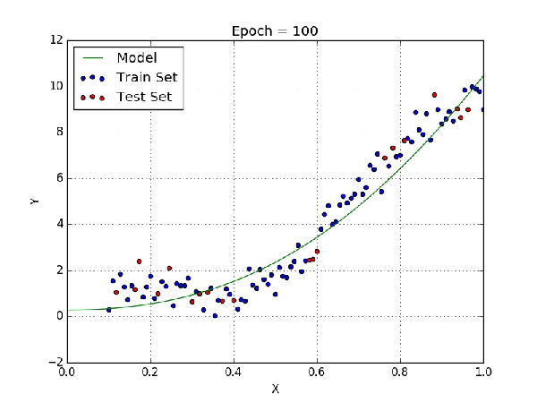
Epochs refer to the amount of data that is being trained by the neural network. Essentially, just know that as the epoch increases, more inputs and outputs are being fed into the neural network model, which will cause the model to fine-tune these "weights" to best model the relationship between inputs and outputs.

This is a simple example, where we have one characteristic of inputs and one characteristic of outputs (e.g. modeling the relationship between participation and final grades), so we use a 2D model. From the chapter 3 example, if we want to measure 3 characteristics and their relationship with one final output (final grade), we will need a 4D model.

Example 1: Predicting Crime

Let's generate a random sample of crime data, which will include inputs such as minority demographics, income level, neighborhood, past history, and education level. The output is whether or not there is low, medium, or high crime risk. How does this neural network impact society?

To find the weights that connect inputs to output, we program a neural network with the data above. Once the set of weights are determined, the neural network can take additional inputs, apply its weights, and produce a new predicted output.

Now, we've trained the model to optimize all the weights, or mathematical relationships, between our inputs and outputs. We can now use these weights, take an input, and predict an output.

Let's play around with this model by putting in random inputs (characteristics) for a person and testing if they are low, middle, or high crime risk.

Here, the distribution of importance highlights that the model heavily relies on socio-economic and demographic factors, such as income, education level, and minority status, rather than purely numerical inputs like historical arrests. Let's think: is this ethical?

Example 2: Predicting Heart Disease

Let's find another application of neural networks: healthcare. Every year, neural network applications are becoming increasingly popular and widespread in the medical field, yet, it lacks diversity in terms of demographics. Although the dataset used below is synthetically generated, we are trying to mimick a real-world scenario where the medical data is more significant amongst majority populations (especially male), as compared to underrepresented or female populations. Using the model below, we can explore how a lack of demographic diversity can influence how neural networks interact with society.

Notice how the amount of data for particularly females and low-income populations are less than those of other demographics.

Once again, using the following sets of inputs and outputs, we can train a model of weights that are responsible for output predictions:

Let's play around! Use the sliders below to choose the demographic of a patient and their characteristics. How does this affect the prediction?

Conclusion

What are the societal implications of Neural Networks on Society?

The intersection of the mathematical and scientific principles behind neural networks with ethical, social, and humanistic concerns presents a profound challenge. While neural networks excel at identifying patterns and making predictions based on large datasets, their reliance on training data inherently reflects the biases and limitations of those datasets. These biases can have far-reaching implications, particularly when applied to socially sensitive contexts such as crime prediction and healthcare.

In our crime prediction example, the neural network was trained on a dataset that encoded racial bias. By disproportionately associating certain racial groups with higher crime risk, the model perpetuated systemic inequities. The math driving the neural network—its optimization of weights to reduce error—does not inherently recognize the ethical implications of these associations. While the network might achieve high accuracy by mirroring patterns in the training data, the resulting predictions reinforce discriminatory practices, potentially leading to unjust surveillance or policing of marginalized communities. This highlights a critical clash: the objective function of minimizing error in neural networks versus the societal imperative to ensure fairness and equity.

Conversely, in the heart attack prediction example, the training dataset excluded key societal demographics such as sex and instead reflected a population that was disproportionately male. This created a different kind of bias—one of exclusion rather than misrepresentation. The network's predictions were highly accurate for the majority demographic (males) but faltered when applied to the minority group (females). This failure underscores the ethical dilemma of deploying models trained on incomplete or unrepresentative data. It raises concerns about whether models can serve diverse populations equitably if their training is limited to one dominant group.

The mathematical underpinnings of neural networks—such as the optimization of loss functions and the tuning of weights—are agnostic to the social contexts in which they operate. However, their outputs have real-world consequences, particularly when the data reflects societal inequities or lacks inclusivity. In the case of crime prediction, the lack of ethical safeguards allowed the model to perpetuate racial biases. In healthcare, the absence of representative data created a system that prioritized accuracy for one group at the expense of another. These examples illustrate how the pursuit of mathematical accuracy often clashes with the need for ethical responsibility.

The implications extend beyond the immediate predictions of neural networks. They raise questions about accountability: who is responsible for ensuring that models are trained on fair and inclusive data? They also challenge us to consider the societal impact of these technologies—whether they are amplifying systemic inequities or working toward greater equity. By critically examining these issues, we can develop frameworks that integrate ethical considerations into the design and deployment of neural networks, ensuring that the powerful tools of math and science are used in ways that align with societal values and human dignity.