Squid Game Prediction Model
Note: Click the "Run" button to load my project!
Background Information
After watching the popular Netflix series Squid Game, I was excited to catch up on the new season. While enjoying the storyline and complex characters, I became intrigued by how players made choices during the games. I noticed that players approached the games with different strategies. Thus, I began this project to analyze the relationship between a player's debt, age, and game choices using predictive modeling. I plan to explore this relationship in the context of age, risk-taking behavior, alliances, and survival outcomes through a Multi-Output Feed Forward Neural Network.
As a result, our model research question is as follows: How does a player’s age and debt level influence their risk-taking behavior, alliance formation, and likelihood of survival in Squid Game?
Phase 1: Data Collection and Preparation
Data was collected from watching Squid Game on Netflix, Squid Game Wiki, and NamuWiki. Age was the only feature for which I didn’t have complete data, as it wasn't disclosed to viewers. Since exact ages were not available, I estimated players' ages based on their appearance.
Extra Data Collection Notes:
I tracked 10 players across two games in regard to their debt, age, risk scores, alliances, and survival outcomes. Since the Dalgona game was not featured in Season 2, some data points were missing. I filled these missing values with -1 for the following reasons:
✅Maintains numeric consistency, ensuring the model recognizes these as missing without biasing results.
✅ Does not interfere with actual game values (Risk Score is 1–10, Alliance Score starts at 0).
✅ Allows the Neural Network to interpret -1 as "missing" and either ignore it or adjust weights accordingly.
Phase 2: EDA
Think of EDA as follows: it's like reading a map before a journey. It helps you avoid pitfalls, choose the best path, and reach your destination—an accurate, reliable model. Hence, this step is critical.
When collecting my data sets, I separated them into two tables. However, I'll combine them together due to my models goal. It's important to note that age and debt affect all three outcomes (behavior, alliance formation, and likelihood of survival) across games. Combining data allows the model to learn general patterns. It also increases the number of observations, improving model generalization.
Run to view results
Run to view results
Now that we finished cleaning our data, we can analyze it!
Run to view results
Distribution Analysis
The Age Distribution exhibited a multimodal pattern, with distinct peaks around the late 20s, mid-30s, and mid-40s, suggesting that players tend to cluster into specific age groups. This uneven distribution might reflect differing strategies or risk-taking behaviors across age brackets.
The Debt (USD) distribution was heavily left-skewed, with a few players carrying significantly higher debt, potentially leading to disproportionate influence on the model’s predictions. In contrast, both the Risk Score and Alliance Score followed relatively normal distributions, making them well-suited for modeling without transformation. To ensure fair representation across age groups, it may be beneficial to either standardize the age feature or group players into age brackets. Overall, the dataset is now prepared for modeling, with attention required to prevent skewed features from distorting the outcomes.
Solution
Standardize Age and Debt, so that the model has data following a normal distribution. This will improve my model's performance by ensuring that all features are on a comparable scale. This also helps avoid any single feature from dominating the learning process.
Run to view results
Box Plot
Run to view results
Analysis
We will begin analyzing the box plots. There are no significant outliers in the age distribution. As a result, this feature will not negatively impact the model's training.
Moving along, there is a clear outlier above the whiskers in the Debt feature. This indicates that one player has significantly higher debt compared to others. Since debt is a key variable for the model, this outlier could have skewed the model's learning and caused it to weigh debt more heavily than necessary when evaluating other features. However, since the features were standardized earlier, the skewness in this feature will not negatively impact the model.
We will ignore the box plots for the Risk and Alliance scores because these are fixed categories with limited possible values. As a result, box plots are not particularly useful for analyzing their distributions. Instead, we will use bar charts, which provide a clearer representation of these categorical features.
Additionally, it is important to note that the debt feature is skewed to the right, as indicated by the median line being closer to the bottom of the box. However, the standardization process has already mitigated any potential issues arising from this skewness.
Run to view results
The distribution of the Alliance Score appears imbalanced, with more observations in the 0 category compared to 1. While the shape may resemble a left-skewed curve, it's important to note that this is categorical data, not a continuous distribution. Therefore, interpreting skewness in the traditional sense may not be entirely appropriate. However, this imbalance is unlikely to negatively impact the model's training or introduce bias toward one side, especially given the categorical nature of the variable.
Run to view results
The distribution of the Risk Score appears skewed to the left, with most data concentrated around the values -1, 2, 4, and 8. This imbalance suggests a need for standardization to ensure the model does not place disproportionate importance on these values during training. If left untransformed, the model might incorrectly prioritize scores like -1, 2, 4, and 8 while underweighting scores like 5 and 7.
It's important to note that the Risk Score has specific categorical meanings:
Low Risk (1-4): Cautious gameplay
Medium Risk (5-7): Balanced risk and safety
High Risk (8-10): Significant risk-taking
The score of -1 signifies missing data rather than an actual risk level. Without transformation, the model might misinterpret -1 as a negative risk score, skewing its learning. Standardizing this feature will provide balance and prevent the model from assigning undue significance to specific values, ensuring more accurate predictions (which has been done above).
Missing Values
Missing values will be replaced with 0 instead of -1 due to features being standardized. This ensures alignment with the mean-centered distribution of all features.
Run to view results
Class Imbalance
Run to view results
Based on the graph above, we only have one class. Hence, there isnt any class imbalance.
Note:
We check for class imbalance to ensure that our model learns to predict all classes accurately, rather than being biased toward the majority class. Class imbalance happens when one class significantly outnumbers another in the target variable.
This matters because:
1. Bias Toward Majority Class: If 90% of the data belongs to class 1 and 10% to class 0, the model might predict 1 all the time and still achieve high accuracy, but it would fail to identify the minority class
2. Poor Generalization: An imbalanced model may struggle with real-world data, where minority class examples are often the most critical to predict.
3. Misleading Metrics: Accuracy can be deceptive. If a model predicts 95% accuracy but ignores the minority class, it's not truly effective.
Feature Scaling
We'll now analyze data to do feature scaling.
Run to view results
Looking at all the features, we want to ensure that the mean is close to 0 or the SD close to 1. This confirms our features are standardized. Notice that the Alliance Score has a mean of .3 and SD of .47. This is perfectly fine as the Alliance Score had a roughly normal distribution, so standardizing it isn't necessary. We know that Alliance Score is roughly normal distributed due to the bar chart built above.
Phase 3: Building the Multi-Output ML Model
Now that we are done analyzing our data, we can build our model!
Run to view results
Side Note:
Mean Squared Error (MSE) measures the average squared difference between the predicted and actual values.
Run to view results
Note:
A couple of red flags have appeared regarding my model’s performance. First, in 4 out of the 16 validation folds, the MSE is greater than or equal to 1. Since we used K-Fold Cross-Validation, this suggests that the model is struggling to generalize well across different data splits. This could indicate high variance in the dataset, sensitivity to certain data partitions, or potential outliers affecting some folds.
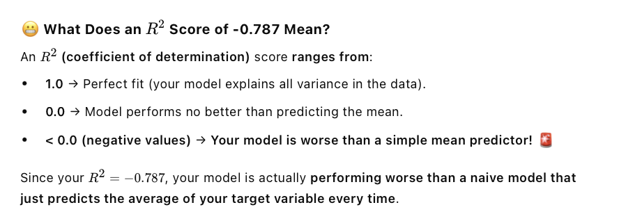
Additionally, the final test R^2 score is negative (−0.8006), meaning the model performs worse than simply predicting the mean of the target variable. To diagnose the issue further, I will plot the validation MSE across the 16 folds to identify patterns and determine whether specific folds are contributing disproportionately to the poor generalization.
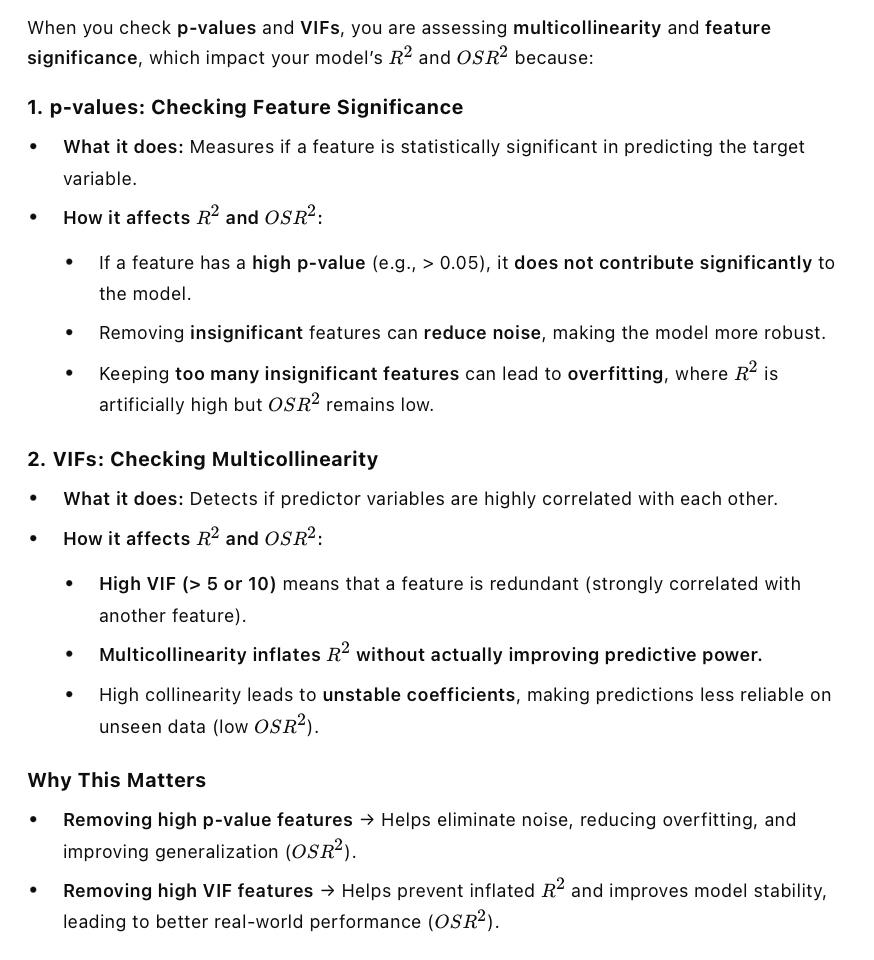
Lastly, I also calculated the OSR^2. I found that its negative. A negative OSR^2 means that my model performs worse than a simple baseline predictor on unseen data, which is a serious problem. In attempt to fix this (and my R^2), I calculated the p-values and VIFs to begin removing variables that arent significant to the model.
Checking p-values and VIFs is important because they help identify irrelevant or redundant features that can artificially inflate R^2 while harming OSR^2. Removing these features can potentially lead to a more stable and generalizable model, improving real-world performance.
Run to view results
After plotting, it's evident that folds seven, eight, nine, and eleven are the ones that contributing to the poor generalization. On the other hand, however, most folds have a low MSE (below 1), which is a good sign of consistent performance. This is not to say that the model is perfect, rather to point out its strengths and weaknesses.
Feature Removal, P-Value Checks, OLS Tests
Run to view results
Run to view results
Running the VIFs and p-values provided valuable insight into why my model is performing worse than baseline. After calculating the VIFs for my two input features (Age and Debt (USD)), I found that both have a VIF of 1.188489. This indicates low or no multicollinearity, meaning these variables are not highly correlated with each other or with other predictors in the dataset.
Since VIF is low, there is no immediate reason to remove these variables based on multicollinearity alone. However, before making a final decision, I need to check their p-values to determine their statistical significance in the model. The p-values will reveal whether these features have a meaningful impact on predicting my output variable.
To assess this, I will run an Ordinary Least Squares (OLS) regression, which will provide p-values and further insights into the relationship between these predictors and the target variable.
Running OLS, we found that Age is only significant for predicting Survival Outcome (p = 0.004), while Debt is not significant for any output variable. This indicates that our current features do not adequately predict Risk Score or Alliance Score, meaning we need additional relevant features to improve model performance. I will dive into this more in Phase 4.
Side Note:
Typically, OLS (Ordinary Least Squares) regression is run on a single output variable (dependent variable). Because I chose a model thats working with multiple output features, running OLS on each output separately can provide insights into how well the independent variables explain different aspects of my dataset.
Important Metric Information
Interpreting MSE
✅ Low MSE → Good model performance
Predictions are close to actual values.
Model is learning well and generalizing.
⚠️ High MSE → Poor model performance
Predictions are far from actual values
Model might be underfitting (too simple) or overfitting (memorizing training data but failing on new data).
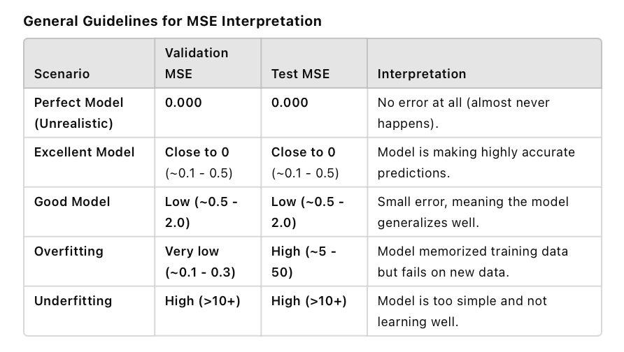
High R^2
P-Values/VIFs
Phase 4: Insights and Conclusions
Its important to note that the initial research question for my project was the following: How does a player’s age and debt level influence their risk-taking behavior, alliance formation, and likelihood of survival in Squid Game?
Based on my analysis, I found that a player’s Age and Debt Level do not strongly predict their Risk Score (risk-taking behavior) or Alliance Score (alliances formed), as indicated by high p-values and weak model performance. This suggests that factors beyond just financial debt and age might influence these decisions in Squid Game.
However, Age showed some significance in predicting Survival Outcome, meaning that age might play a role in a player's likelihood of survival. The direction of this relationship requires further exploration—older players may have more experience, while younger players may have more physical endurance. Overall, my findings indicate that Age and Debt (USD) alone are insufficient to explain risk-taking, alliances, and survival outcomes. Future iterations of this model should explore additional features, such psychological factors, to better understand survival in Squid Game.
Model Improvements
When I initially ran my MLP test model, I noticed that three validation folds had MSE values above 1, with one extreme outlier reaching an MSE of 304. Recognizing this as a red flag, I used K-Fold Cross-Validation to analyze and address the issue. To improve performance, I made several adjustments to the model’s architecture and hyperparameters. First, I increased the hidden layer sizes from 80 and 30 to 128, 64, and 32, allowing the model to capture more complex patterns. Additionally, I lowered the learning rate from 0.2 to 0.003 to stabilize weight updates and prevent erratic fluctuations. I also decreased the batch size from 14 to 10 to align more closely with my dataset, which consisted of 20 data points, ensuring that mini-batch gradient updates remained effective. Furthermore, I reduced the maximum number of iterations from 500 to 400, striking a balance between sufficient training and avoiding unnecessary overfitting.
After these adjustments, the extreme outlier MSE of 304 significantly decreased to 4.510, representing a 98.5% reduction in the worst-case validation error. While the number of validation MSEs above 1 increased from three to four, one of these values is now approximately 5 (compared to the previous 304), while the remaining three are under 1.5. These improvements highlight that, although the distribution of errors slightly shifted, the overall consistency and stability of the model improved substantially. The refined model now generalizes better across validation folds, showing that lowering the learning rate, increasing layers, and optimizing batch size helped achieve lower validation errors. Additionally, experimenting with different solvers confirmed that Adam provided the best stability and convergence. Although increasing layers and iterations extended training time, the trade-off was worthwhile as it significantly reduced extreme errors and enhanced predictive accuracy. These changes transformed the model into a more reliable system with a much lower overall MSE.
In attempt to improve my model, I began the process of analyzing p-values and VIFs. I found that running OLS on each of my dependent variables gave me insight as to how these features arent helpful for my model. I arrived at this conclusion based on the p-values not being significant, as Im using a 95% CI. Age and Debt (in USD) had little to no outcome in the predictions for Alliance Score and Risk Score. However, these features were found to be significant for predicting Survival Outcome. VIFs were ~2 for the independent variables, indicating that there isnt multi-collinearity. This ensures that the model isnt being provided with redundant information, making it easier for it to separate the individual effects on the dependent variable.
Currently, my model is doing worse than baseline. R^2 and OSR^2 provided me this insight as theyre both negative values. To solve this, I'll cover four strategies Id implement if time permitted. This will be mentioned below.
Improving Model Performance (if I had more time)
In this project, I standardized two input features (Age and Debt in USD) and one output feature (Risk Score) to handle skewness and improve model performance. A key consideration when standardizing target variables is that predictions must be inverse-transformed to return to the original scale. For future iterations, I would ensure that standardization is applied only to the training set before splitting. Furthermore, I would implement the following strategies to improve model performance:
1. Expand Feature Selection: Include more variables, such as psychological profiles.
2. Increase Data Collection: A more diverse dataset could help capture patterns that aren’t evident in a smaller sample.
3. Try a Different Model Type: A tree-based model (Random Forest, XGBoost) might detect non-linear relationships that a feedforward neural network may have missed.
4. Analyze Interaction Effects: Instead of treating Age and Debt separately, I’d explore how they interact—e.g., do older players with high debt take more risks than younger players with high debt?
Since this is a side project, I am documenting these insights for future reference while moving forward to a new project.
Deployment (if I had more time)
Once I was satisfied with my model’s performance and it was meeting all the metric standards, I would proceed with deploying it. Deployment would look as follows: I’d save the trained model so it can be reused. Then, I’d create a simple system where people or apps could send data to the model and receive predictions. Next, I’d put it online using a cloud service so it’s always accessible without needing my computer to be on. If needed, I could connect it to a website or app to make it user-friendly. Finally, I’d monitor its performance and update it over time to improve accuracy.
Conclusion
I had a great time building this model. Even though it didn’t meet the expected performance metrics, I learned a lot about EDA, fine-tuning hyperparameters, and transforming data to optimize the model's performance. Diagnosing and pinpointing why my model wasn’t performing well in terms of R² and OSR² allowed me to take a step back and see the bigger picture. Understanding that model creation is an iterative process helped me appreciate the beauty of improving models as more data and analysis uncover issues affecting performance. The good news is that these challenges can be resolved with more time and refinement. Overall, I loved this project and look forward to building future models!