Capstone Project - Reel Analytics


Authors:
Part 0: Introduction
0.1 Project Overview
0.2 How it started
0.3 Reel Analytics Overview
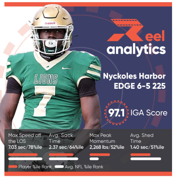
Figure 0.3.1 - RA Grading Card (Rights and Source: https://reel-analytics.net/)
0.4 Project Scope
0.5 Reel Analytics Data
0.6 Pro Football Focus (PFF) Data
0.7 CollegeFootballData (CFBdata)
Part 1: Labeling the Data
1.0 PFF Data import & processing
Figure 1.0.1 - College Divisions Performance Factors
1.1 Player Ranking
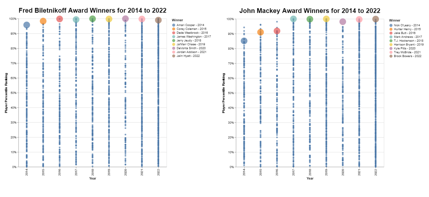
Figure 1.1.1 - Ranking of both Fred Biletnikoff and John Mackey Winners - 2014 to 2022
1.2 UMAP dimensionality reduction
Figure 1.2.1 - UMAP 2D projection of PFF data
1.3 KMeans Cluster Analysis
Figure 1.3.1 - Number of Cluster Evaluation
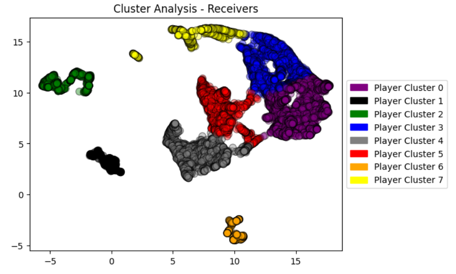
Figure 1.3.2 - Number of Cluster Evaluation
For each of the selected clusters, we analyzed their overall ranking distribution, as seen in Figure 1.3.3. Then, to gain a deeper understanding of these clusters' characteristics, we then extracted their prominent features. This process allowed us to identify the key factors influencing their respective rankings. Here is their respective analysis:
Cluster 3 - Elite Wide Receivers
Cluster 7 - Penalty Magnets/Disruptors
Cluster 5 - Stereotypical & Efficient Tight Ends
Figure 1.3.3 - Cluster Analysis: Ranking Distribution
Figure 1.3.4 - John Mackey Winners Through Clusters
Figure 1.3.5 - Fred Biletnikoff Winners Through Clusters
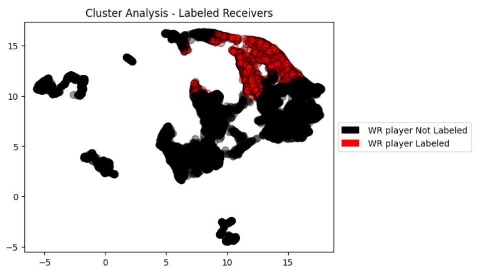
Figure 1.3.6 - Cluster Analysis - Labeled Receivers
Part 2: Modeling the Data
Our objective was to create a logistic regression model to predict if a player from the RA database will be a successful Wide Receiver in college.
2.0 Combining and Cleaning
To do this, we started with the PFF dataset and applied the clustered label from Part 1 as our target label. With the sparse RA data lacking features to help differentiate players of the same name, we utilized the CollegeFootballData recruit data to add a few additional players to our data frame used for the model.
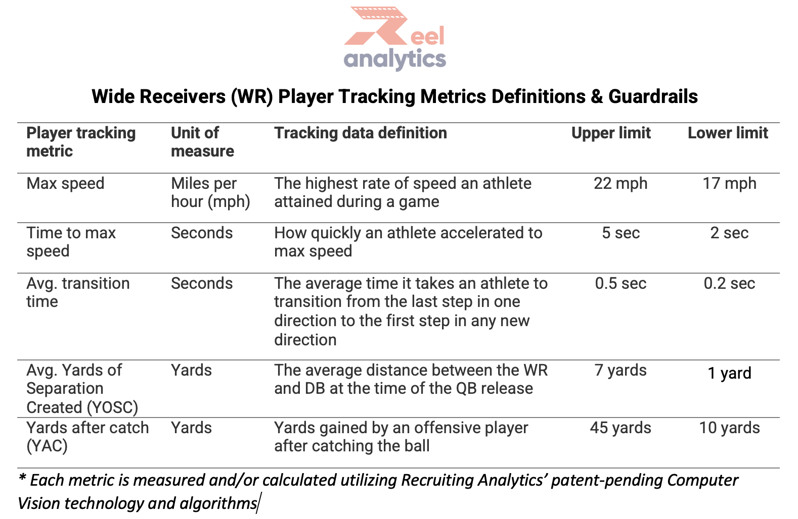
The next step in cleaning the data frame was to apply thresholds based on RA's documentation (image below). The player data included many data points that fell outside of the provided max and min range for each of the measured athletic scores. To address this, we applied a percentile replacement value for any point that was above or below the threshold.
2.1 Challenging Data
Figure 2.1.1 - Reel Analytics Data by Year
Additionally, and as mentioned before, the RA dataset lacks certain player features that would help in matching with other datasets we're using. For example, the school they committed to or attended and anything about where they played their High School football is absent. These characteristics also led to a shrinking of our usable data pool, as many players with common names were unable to match uniquely.
The funnel below visualizes the fallout we experienced with the dataset used for modeling.
Figure 2.1.2 - Data Fallout
2.2 Modeling the Data
With our smaller-than-desired data set of ~2.3k wide receivers, we used a 70 / 30 split for training and testing. Due to the unbalanced labels in our data of successful versus not successful college players, we implemented oversampling techniques to help assist the model. First, we used RandomOverSampler and then passed the data through SMOTE (Synthetic Minority Over-sampling Technique). Both of these packages have different approaches in combating class imbalance but focus on including additional samples to create a better balance. Of note, without these two inclusions, the model was not returning any positive predictions.
The logistic regression model was then created, using a penalty of L2 and a class weight of ‘balanced’ to further help with the class imbalance (shown in Figure 2.2.1). From here, we fed this model into GridSearch to help identify the best value for C (0.01) while cross-validating five times.
Figure 2.2.1 - Mathematical Formula of our Logistic Model
2.3 Judging the Data
With our logistic regression model fit and predicting outcomes for our test data, it was time to see its performance. To judge this, we settled on using the F1-score as our main metric due to its ability to capture both precision and recall for predictions with our class imbalance.
Here we've printed a classification report to easily show the metrics for each outcome, with an F1-score of .62 pointing towards acceptability for our model given all of the constraints we faced.
Figure 2.3.1 - Predicted and Actual Labels by Year
Part 3: Recreating the IGA Score
3.1 Feature Weighting
Now that the weights are linear, the next step was to normalize them in order to work toward a number that would also be on a 100-point scale.
We've included the Reel Analytics weights for direct comparison. Our score is more balanced across the five features than RA's.
3.2 UM IGA Score
Next, we multiplied every player's measurement into a percentile rank based on the normalized feature weight above. The last step was to sum up the five scores for each player and multiply by 100 to achieve our unbiased UM IGA Score.
A preview of our output is below, with the highest scores showing.
Part 4: Comparing IGA Scores
Figure 4.1.1 - IGA Score Distributions
Figure 4.1.2 - Prediction Variance Distribution