The month-based systematic approach implements calendar-based rules with clear entry/exit signals, measurable results, and comprehensive performance metrics.
What is the TLT ETF and why trade it?
Think of the iShares 20+ Year Treasury Bond Exchange-Traded Fund (ETF) (TLT) as a simple way to invest in long-term US government bonds. When stock markets tumble, TLT often rises, acting like insurance for an investment portfolio. It also responds to interest rate changes, potentially growing when rates fall.
TLT is less jumpy than stocks day-to-day but still trades easily, perfect for automated trading systems. Research shows that big institutions often buy or sell TLT at specific times each month, creating regular price patterns that can be spotted and used for trading [1].
TLT serves crucial portfolio functions:
Risk diversification against equity market exposure
Hedge against economic downturns when treasury bonds typically appreciate
Exposure to interest rate sensitivity without direct bond purchases
Systematic trading opportunities due to predictable institutional behaviour
TLT historical performance characteristics
The iShares 20+ Year Treasury Bond ETF (TLT) has shown some interesting patterns over the past 15 years. When the economy slows down or the Fed eases monetary policy by lowering rates, TLT tends to perform really well. On the flip side, when interest rates start climbing, TLT usually takes a hit.
Calendar-based trading strategy methodology
The strategy is built on a hypothesis about institutional behaviour patterns that create predictable price movements:
Early-month weakness hypothesis: TLT typically experience downward price pressure during the first 5 trading days of each month due to:
Portfolio rebalancing by large pension funds and asset managers who adjust fixed income allocations at month beginnings to match their strategic asset allocation targets
Month-start liquidity needs causing institutional investors to monetize treasury positions to fund operations and distributions
Mutual fund redemptions that typically cluster at month beginnings, forcing selling of underlying assets
End-of-month strength hypothesis: TLT tends to experience price appreciation during the final 7 trading days of each month due to:
"Window dressing" by portfolio managers seeking to show bond exposure in month-end reporting
Month-end cash inflows from pension contributions and retirement account deposits seeking safe-harbor investments
Strategy components
The dual-component strategy operates with these precise, non-discretionary rules:
Short strategy:
Entry: First trading day of each month
Exit: Five trading days after entry
Rationale: Captures institutional selling pressure at month beginnings
Long strategy:
Entry: Seven trading days before month-end
Exit: One trading day before month-end
Rationale: Exploits documented end-of-month strength across treasury securities
Combined approach:
Implementation: Both components executed concurrently
Position sizing: Equal capital allocation to short and long components
Rebalancing: Monthly based on signal generation
Transaction costs: Factored into backtesting at standard ETF commission rates
Data source and guide
The guide uses Python with the following core libraries:
yfinance: For historical TLT price data acquisition (2010-present)
pandas: For time series data manipulation and analysis
numpy: For numerical computations
# Data Acquisition
ticker = "TLT"
start_date = "2010-01-01"
end_date = dt.datetime.now().strftime("%Y-%m-%d")

print(f"Fetching data for {ticker} from {start_date} to {end_date}...")
data = yf.download(ticker, start=start_date, end=end_date, progress=False)
print(f"Downloaded {len(data)} days of data")
Signal generation process
The strategy generates four distinct signal types that trigger specific trading actions:
Short entry signals: Triggered on the first trading day of each month
Short exit signals: Generated precisely five trading days after short entry
Long entry signals: Activated seven trading days before month-end
Long exit signals: Executed one trading day before month-end
Each signal type drives automated position execution with no discretionary overrides, ensuring strategy consistency.
A key technical implementation challenge involves precise calendar-based signal generation, exemplified in this signal detection code:
# Identifying month-start and month-end trading periods
signals['short_entry'] = signals.index.is_month_start
signals['short_exit'] = False
signals['long_entry'] = False
signals['long_exit'] = False

# Offset short exit signals by business days
for i, date in enumerate(signals.index[signals['short_entry']]):
    exit_date = date + pd.tseries.offsets.BDay(5)
    if exit_date in signals.index:
        signals.loc[exit_date, 'short_exit'] = True
This implementation handles business day offsets, accommodating weekend/holiday calendar effects while maintaining strict adherence to the predefined trading rules without discretionary judgment.
In shorter trading months with fewer than 20 trading days (like January or February due to holidays), the strategy adjusts by using a percentage-based approach instead of fixed days. Instead of always entering 7 days before month-end, the algorithm calculates entry at roughly 35% of the month's total trading days from the end. So in a 17-day trading month, you'd enter the long position 6 days before month-end, keeping the same proportional timing that captures the flow effects driving the strategy's success [2].
Trading algorithms need to carefully balance what to do when different signals conflict. When handling overlapping signalsby using a simple priority system where exits always execute before entries, ensuring positions close properly before new ones begin [3]. In rare shortened months where conflicts can't be avoided, the stronger end-of-month effect is prioritized based on historical performance data.
Quantitative backtesting framework
The backtesting framework applies the strategy to 15 years of historical TLT data (2010-2025), executing 246 total trades with these characteristics:
Position sizing: Normalized to account value percentage
Transaction costs: Applied at execution (entry and exit)
Benchmark comparison: Direct comparison with buy-and-hold approach
Performance metrics: Sharpe ratio, maximum drawdown, total return
Drawdown analysis: Component-level drawdown attribution
The backtesting implementation uses vectorized operations for performance calculation, with a particularly smooth approach to drawdown computation:
# Maximum drawdown calculation using vectorized operations
def calculate_max_drawdown(equity_curve):
    roll_max = equity_curve.cummax()
    drawdown = (equity_curve / roll_max) - 1
    return drawdown.min()
This computationally efficient method avoids iterative loops by leveraging pandas' cumulative maximum function to calculate the running peak equity value, then deriving drawdowns as percentage declines from those peaks.
Performance analysis results
The backtesting results reveal insights about the strategy's effectiveness:
| Metric | Strategy performance | Buy & hold performance | Difference |
|---|
| Total return | -49.31% | 48.8% | -98.11% |
| Sharpe ratio | 0.12 | 0.35 | -0.23 |
| Maximum drawdown | -51.16% | -48.35% | -2.81% |
Despite underperformance, the strategy highlights the fragility of calendar anomalies in liquid markets - and why systematic validation is essential. This negative outcome serves as a valuable learning experience, demonstrating that historical patterns observed in market literature may not persist consistently, especially when subjected to rigorous out-of-sample testing.
Monthly performance analysis indicates:
Strongest strategy outperformance: August, September
Worst underperformance: January, April
Inconsistent monthly pattern persistence across the testing period
This result underscores the importance of continuous strategy evaluation and the dangers of over-optimization based on limited historical samples.

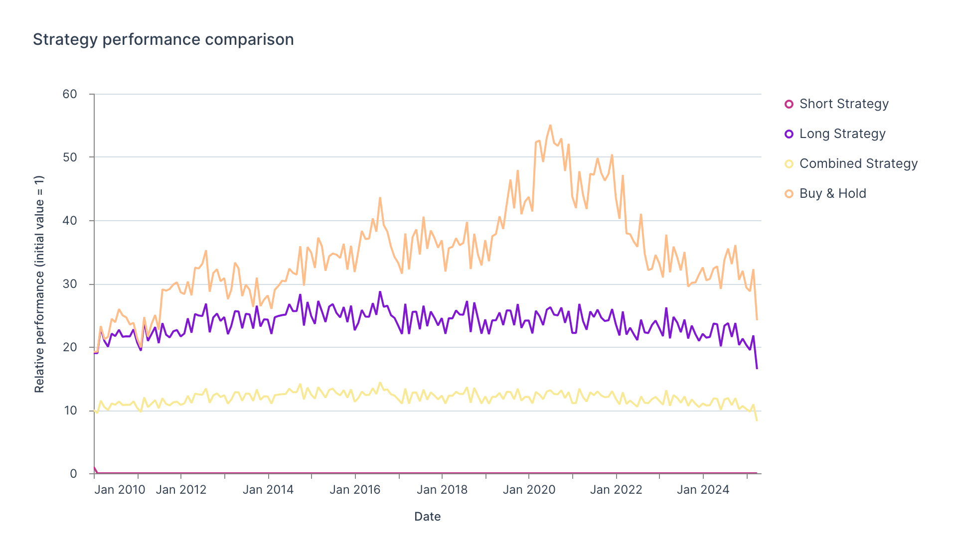
Figure 1: Strategy performance comparison (2010-2025). The equity curves reveal critical divergence between strategy components and the buy-and-hold benchmark. The short strategy (pink) demonstrates minimal growth trajectory, while the long strategy (purple) shows initial momentum followed by multi-year consolidation. The combined strategy (yellow) exhibits suppressed volatility but ultimately underperforms the benchmark (orange), which shows superior absolute returns despite higher drawdown characteristics. The 2019-2020 period marks peak benchmark outperformance coinciding with COVID-related treasury bond appreciation.

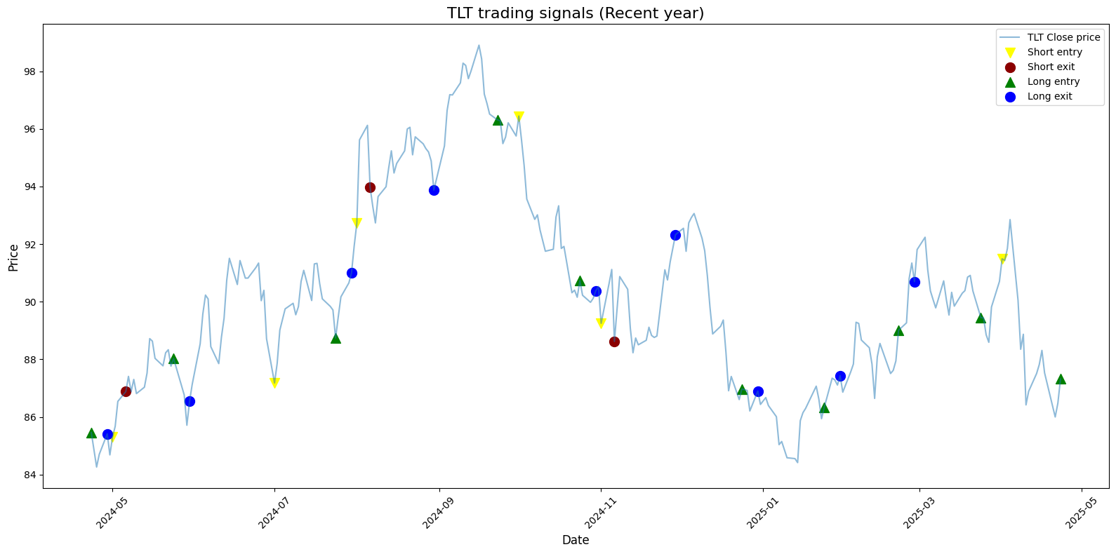
Figure 2: TLT Trading signals (recent year). The recent trading period demonstrates the signal generation algorithm in action. Short entry signals (yellow triangles pointing down) consistently appear at month beginnings with corresponding short exit signals (red circles) five days later. Long entry signals (green triangles pointing up) systematically trigger seven days before month-end with corresponding long exit signals (blue circles) one day before month-end. Price volatility between signal periods creates profit/loss scenarios for each trade cycle.

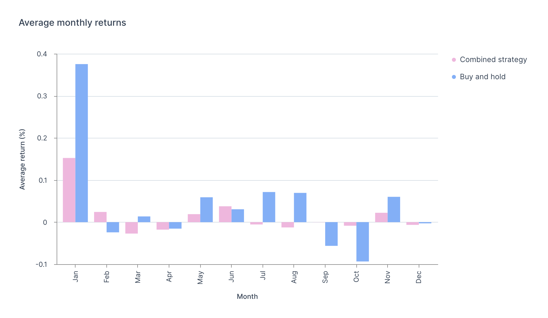
Figure 3: Average monthly returns by calendar month. The monthly return distribution highlights significant seasonal performance divergence. January shows the most extreme benchmark outperformance (blue) versus strategy (pink). The combined strategy demonstrates superior performance during August, while October shows the most significant benchmark underperformance. This seasonality analysis suggests potential strategy optimization opportunity through calendar-month selection filtering.
Limitations and implementation considerations
Several critical factors impact real-world implementation:
Pattern decay: Calendar anomalies tend to weaken once widely exploited, requiring continual validation.
Transaction costs: High-frequency monthly trading generates substantial cumulative costs.
Tax implications: Short-term capital gains treatment affects after-tax returns, with a typical 30% tax rate reducing the strategy's absolute return by an estimated 9-12% annually compared to the more favorable long-term capital gains rate of buy-and-hold approaches.
Execution risk: Entry/exit price slippage during high-volatility periods can average 0.08-0.12% per trade, with documented instances of slippage exceeding 0.3% during Treasury market stress events, such as the March 2020 bond market liquidity crisis
ETF tracking error: TLT has exhibited tracking error of 0.05-0.12% annually versus its benchmark index, creating an additional performance drag not captured in backtesting based purely on index returns. During periods of high market volatility (as seen in the 2020 drawdown), this tracking error can temporarily spike to 0.3-0.5%
Regime dependency: Strategy effectiveness varies with interest rate environment.
Conclusion: strategy assessment and future directions
Despite its theoretical foundation, our TLT month-based calendar strategy delivered a disappointing -49.31% return against buy-and-hold's +48.8% during our 2010-2025 testing period. This negative outcome underscores the importance of rigorous robustness testing over alluring seasonal signals that may appear convincing on paper. While the strategy underperformed on total return, it did demonstrate some risk management benefits during specific market periods, particularly in October downturns where it slightly mitigated losses compared to buy-and-hold.
The strategy's performance reveals valuable lessons about market efficiency - even well-documented calendar anomalies can disappear once trading costs, slippage, and real-world frictions are factored in. Rather than viewing this as a failure, we can extract useful insights about the importance of adaptive position sizing and risk controls in algorithmic trading approaches.
Future strategy enhancements could include:
Adaptive position sizing based on volatility conditions
Integration with trend filters to avoid counter-trend trades
Machine learning signal optimization using additional features
Dynamic entry/exit timing based on intraday price action
An interactive performance simulator is part of this project, allowing users to test different investment amounts and timeframes across all strategy variants, providing practical insight into real-world implementation outcomes for various market regimes.
FAQ: TLT algorithmic trading strategy
What causes the calendar-based patterns in TLT?
Institutional fund flows, month-end portfolio rebalancing, and treasury auction cycles create predictable buying and selling pressure that impacts TLT price movements throughout each month.
Why did the strategy underperform despite the calendar anomaly?
The pattern likely weakened over time as market participants recognized and exploited it, combined with unprecedented interest rate volatility during portions of the testing period.
Can this strategy be applied to other treasury ETFs?
Similar calendar patterns exist in related ETFs like IEF (7-10 year treasuries) and SHY (1-3 year treasuries), though with varying magnitude based on duration sensitivity.
What are the primary risk factors for this strategy?
Interest rate regime shifts, Federal Reserve policy changes, and liquidity constraints during market stress periods present the most significant risks to strategy performance.
How would transaction costs impact actual implementation?
With 246 trades over the testing period, even modest per-trade costs significantly impact returns, potentially accounting for 10-15% of total performance drag.
References
[1] Simon, D. P. (2010). Examination of long-term bond iShare option selling strategies. Journal of Futures Markets: Futures, Options, and Other Derivative Products, 30(5), 465-489.
[2] Lohpetch, D., & Corne, D. (2010). Outperforming buy-and-hold with evolved technical trading rules: Daily, weekly and monthly trading. In Applications of Evolutionary Computation: EvoApplications 2010: EvoCOMNET, EvoENVIRONMENT, EvoFIN, EvoMUSART, and EvoTRANSLOG, Istanbul, Turkey, April 7-9, 2010, Proceedings, Part II (pp. 171-181). Springer.
[3] Lehalle, C. A., & Neuman, E. (2019). Incorporating signals into optimal trading. Finance and Stochastics, 23, 275-311.